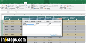
Excel "excels" at sorting and filtering columns based on cell content, including advanced features like coloring rows based on rules ("conditional formatting"), grouping rows by unique value, etc. It's really easy (and useful!) to learn how to sort spreadsheets alphabetically / numerically, how to invert the current sort order, or even sorting each row from a list of custom values. Note: I'm using Excel 2016, but this tutorial also applies to Excel 2013 / 2010 / 2007!
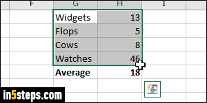
Start by selecting the cells you want to sort: how to select rows / columns. If your data spans multiple columns, select all relevant rows and columns. (I didn't select the last row, because it contains a formula to calculate the average!)
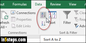
Now select the "Data" tab in the ribbon. To sort a single column, click on the "A-Z" button to sort in increasing order (alphabetically, and from small to large if the column contains numbers). To reverse the sort to inverse alphabetical order, or to go from large to small, click on the "Z-A" button instead!
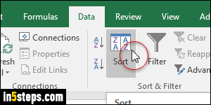
To sort multiple columns based on one column's values (and keep all related rows together!), click on the big Sort button, as I did on the screenshot.
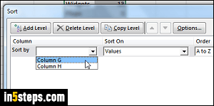
Under "Column", select the column letter: if you labeled your columns, Excel will show their names in the dropdown. Leave "Values" selected under "Sort On". Under "Order", pick A to Z for ascending order, or Z to A for descending order. To sort any other way (like by month or week day), pick "Custom List" and create a new list, or use an existing one. Click OK to apply the sort!
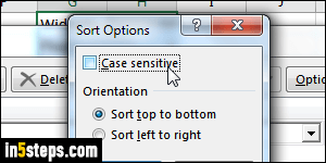
Bonus Tip - Sort case-sensitively, and sort by row!
In the Sort popup from Step 5, you can click on the Options button to make Excel sort case-sensitively (where capitalization matters, and uppercase comes before lowercase). You can also "sort left to right" to sort by row (horizontally), instead of the default "Sort top to bottom" to sort vertically, by column!

